YOLOv3 Network Architecture

YOLO network accepts an image of fixed input dimension. In theory, YOLO is invariant to the size of the input image. However, in practice, the input image were resized to a fixed dimension of 512 by 512 to process images in batches and train the network faster.

YOLOv3 uses a variant of the custom deep architecture Darknet, originally 53-layer network trained on Imagenet with 53-layer stack added for the task of detection for a total of a 106-layer fully convolutional underlying architecture for YOLOv3. Thus, the runtime of YOLOv3 is much slower compared to the runtime of YOLOv2 in addtion to YOLOv4 and YOLOv5.

The newer architecture boasts of residual blocks, skip connections, and upsampling. The most salient feature of YOLOv3 is that it makes detections at three different scales. YOLO is a fully convolutional network and its eventual output is generated by applying a 1 by 1 kernel on a feature map. In YOLO v3, the detection is done by applying 1 by 1 detection kernels on feature maps of three different sizes at three different places in the network.

The shape of the detection kernel is 1 x 1 x (B x (5 + C)) where B is the number of bounding boxes a cell on the feature map can predict, C is the number of classes, and the constant of 5 is for the four bounding box attributes and one confidence/objectness score. For the DD dataset, B = 3 and C = 3 such that the kernel size is 1 by 1 by 24. The feature map produced by this kernel has identical height and width of the previous feature map, and has detection attributes along the depth as described above.

YOLOv3 makes prediction at three scales by downsampling the dimensions of the input image by a stride of 32, 16, and 8 respectively. The first detection is made by the 82nd layer. The resultant feature map is 16 by 16 where a detection is made using the 1 by 1 detection kernel for a detection feature map of 16 by 16 by 255. The second detection is made by the 94th layer for a detection feature map of 32 by 32 by 255. The third and final detection is made by the 106th layer for a feature map of 64 by 64 by 255. Detections at different layers helps address the issue of detecting small objects. The upsampled layers concatenated with the previous layers help preserve the fine grained features which help in detecting small objects. The 16 by 16 layer is responsible for detecting large objects, the 32 by 32 layer detecting medium objects, and the 64 by 64 layer detecting small objects.

For an input image of same size, YOLOv3 predicts more bounding boxes than YOLOv2. For an input image of 512 by 512, YOLOv2 predicts 1,280 boxes where five boxes are detected using five anchors at each grid cell. However, YOLOv3 predicts 16,128 boxes or 10 times the number of boxes versus YOLOv2 where it predicts boxes at three different scales and predicts three boxes using three anchors at each scale for a total of nine boxes. Thus, YOLOv3 is also much slower than YOLOv2.

The number of bounding boxes near the region where the object is located will have many boxes persisting even after thresholding the confidence/objectness score. YOLO uses Non-Maximal Suppression (NMS) to only keep the best bounding box. The first step in NMS is to remove all the predicted bounding boxes that have a detection probability that is less than a given NMS threshold. The second step in NMS is remove all the bounding boxes whose Intersection Over Union (IOU) value is higher than a given IOU threshold where IOU calculates the ratio of area of overlap to the area of union between two bounding box outputs.

Detection Algorithm

YOLO divides the input image into an S by S grid. If the center of an object falls into a grid cell, that grid cell is responsible for detecting that object. Each grid cell predicts B bounding boxes and confidence scores for those boxes. These confidence scores reflect the confidence of box containing an object and accuracy of the box it predicts. The confidence score is defined as P(Object) x IOU. If no object exists in that cell, the confidence scores should be zero. Otherwise the confidence score is equal the IOU between the predicted box and the ground truth. Therefore, the confidence prediction represents the IOU between the predicted box and any ground truth box.

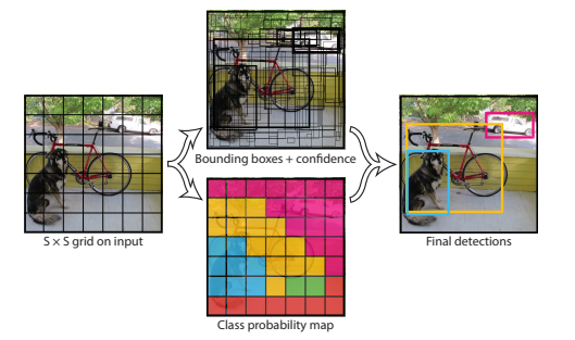
Each grid cell also predicts C conditional class probabilities, P(C_i|Object). These probabilities are conditioned on the grid cell containing an object. Only one set of class probabilities per grid cell is predicted, regardless of the number of boxes B. The class-specific confidence scores for each box is the product P( C_i|Object) x P(Object) x IOU = P(C_i) x IOU. These confidence scores encode both the probability of that class appearing in the box and how well the predicted box fits the object.

Loss Function

YOLOv3 uses sum-squared error between the predictions and the ground truth to calculate the loss. The total loss value from the network is the sum of the classification loss, localization loss, and confidence loss.

The loss function is a combination of the classification loss, localization loss between the predicted bounding box and ground truth box, and the confidence loss. The classification loss is the squared error of conditional class probabilities for each class. Localization loss is calculated between the errors in bounding box centroids and its width and height where smaller bounding boxes are penalized greater than larger bounding boxes for the added precision. The confidence loss is the presence or absence of the object within the bounding box. The loss is calculated for both presence and absence to decrease the confidence when no object is detected and increase confidence when an object is detected.